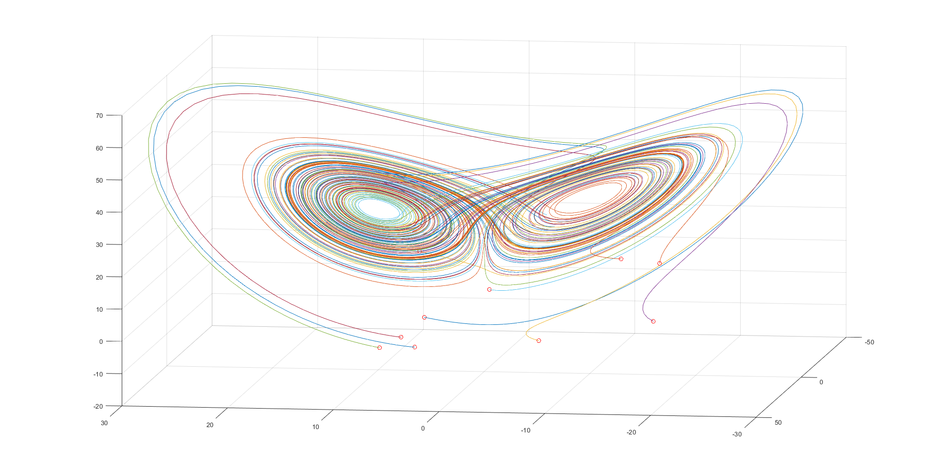
This is Lorenz attractor presented by Edward Lorenz in 1963. The system of equations which leads to get such graphs is called Lorenz system and consist of three non-linear differential equations that modeling in the simplest possible way a phenomenon of thermal convection in the atmosphere. For some set of parameters, the system of ODE equations behaves chaotically, and the plot of variables in the phase space presents a strange attractor. This attractor is the particular solution of Lorenz system and its shape is a little bit similiar to butterfly or figure eight.

This is the Matlab code to generate the plot.

% Atraktor Lorenza
dt=0.005; 
T=10; 
t=0:dt:T;

b=8/3; 
sig=13; 
r=33;

Lorenz_atraktor = @(t,x) ([ sig * (x(2) - x(1)) 
                            r * x(1)-x(1) * x(3) - x(2) 
                            x(1) * x(2) - b*x(3) ]);

NofT = 10; % Number of trajectories (learning data)

% matrices for learning data
input = zeros(NofT * T / dt,3) ;
output = zeros(NofT * T / dt,3) ;
figure
for jj=1:NofT 
    InitConds = (17+17)*(rand(3,1)) - 17;     % initial conditions were created randomly
    [t,y] = ode45(Lorenz_atraktor, t, InitConds);
    input(1 + (jj-1)*(T/dt):jj * T/dt,:) = y(1:end-1,:);
    output(1 + (jj-1)*(T/dt):jj * T/dt,:) = y(2:end,:);
    plot3(y(:,1), y(:,2), y(:,3)), hold on
    plot3(InitConds(1), InitConds(2), InitConds(3), 'ro')
end
grid on

I decided to create neural network in Matlab enviroment and check if it is possible to learn this network solving Lorenz system for parameters in which the system shows the features of chaos.
At the beginning of the program the system of differential equations is solved by the procedure ode45. At the same time, the learning data matrix is created, which will be used to train the neural network. The learning data are simple three numbers, the solution matrix "y" is simply moved 1 row down, the network have to learn how to get the next point P(n+1) from the point P(n).
The initial conditions are random (-17, 17) for each loop execution. Thus, each time the program is compiled, we have new trajectories.

Then, the neural network is subjected to the learning process. At the beginning we need to define network parameters such as network type, number of layers, number of neurons in the layer, learning algorithm and transfer function (also known as activation function). These are the basic parameters. After the learning process, the network is tested. We check how it will cope if we give it completely new data at the input. At this point in the experiment, we can check the performance of the network in many ways, I used a simple criterion - mean square error. The effect of the neural network is compared with the results of the 'ode45' procedure for the same input data.

First step of experiment consisted in defining a 1-layer network with the number of neurons equal to 10 and changing the transfer function. The learning algorithm was chosen arbitrarily. This is the Levenberg-Marquardt algorithm which convergence is the fastest from all algorithms offered by Matlab.

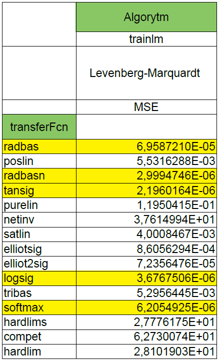
The criterion, of course, was MSE. This led to the generation of a table in which we can check which transfer function copes best with such problem. Parameters of the algorithms have been changed for the necessity of the experiment. The learning process has several conditions that cause its interruption. In order to check clearly the given transfer functions, I introduced several modifications to the parameters of the algorithms. The minimal gradient has been set to 0, the number of iterations has been set to 1000, the maximum number of errors out of range after which the learning process is interrupted has been increased from 6 to 50.

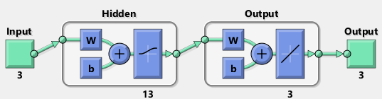
After such experiments I chose the 5 best transfer functions, the 5-layer and 3-layer neural networks were made and the learning process was repeated. The effects compared to the 1-layer network for 5-layer NN are... worse. But for 3-layer NN are better. A bit of confusion will not hurt, right? :)

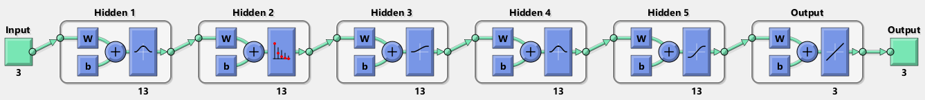
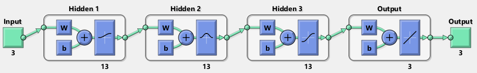
With the 5-layer and 3-layer networks, one more modification has been made: the number of neurons in each layer has been increased to 13.

liczba.warstw = 3;
liczba.neuronow = 13;
LY = liczba.neuronow * ones(1, liczba.warstw);

net = feedforwardnet(LY, 'trainlm'); 

net.layers{1}.transferFcn = 'logsig';
net.layers{2}.transferFcn = 'radbasn';
net.layers{3}.transferFcn = 'tansig';
net.trainParam.min_grad = 0;
net.trainParam.epochs = 1000;
net.trainParam.max_fail = 50;
[net, tr] = train(net, input', output');
view(net)
plotperform(tr)
mse = tr.best_vperf

figure
InitConds = (17+17)*(rand(3,1)) - 17;
[t,y] = ode45(Lorenz_atraktor, t, InitConds);
plot3(y(:,1), y(:,2), y(:,3),'b'), hold on
plot3(InitConds(1), InitConds(2), InitConds(3), 'bo', 'Linewidth',1.5)
plot3(y(end,1), y(end,2), y(end,3), 'bx', 'Linewidth',1.5)
grid on

ynn(1,:) = InitConds;
for jj=2:length(t)
    y0 = net(InitConds);
    ynn(jj,:) = y0'; 
    InitConds = y0;
end
plot3(ynn(:,1), ynn(:,2), ynn(:,3),'r')
plot3(ynn(end,1), ynn(end,2), ynn(end,3), 'rx', 'Linewidth', 1.5)
legend('ode45','InitConds','LastPointODE','neural network','LastPointNN')

figure
subplot(3,1,1) 
plot(t,y(:,1), t, ynn(:,1),'Linewidth',1.5)
ylabel('Współrzędna X');
title('Układ Lorenza');

subplot(3,1,2) 
plot(t,y(:,2),t,ynn(:,2),'Linewidth',1.5)
ylabel('Współrzędna Y');

subplot(3,1,3) 
plot(t,y(:,3),t,ynn(:,3),'Linewidth',1.5)
xlabel('czas [s]');
ylabel('Współrzędna Z');
legend('ode45','neural network');

figure
plot(y(:,1), y(:,2), ynn(:,1), ynn(:,2),'Linewidth',1.5)
legend('ode45','neural network');
title('Rzut XY');

figure
plot(y(:,2), y(:,3), ynn(:,2), ynn(:,3),'Linewidth',1.5)
legend('ode45','neural network');
title('Rzut YZ');

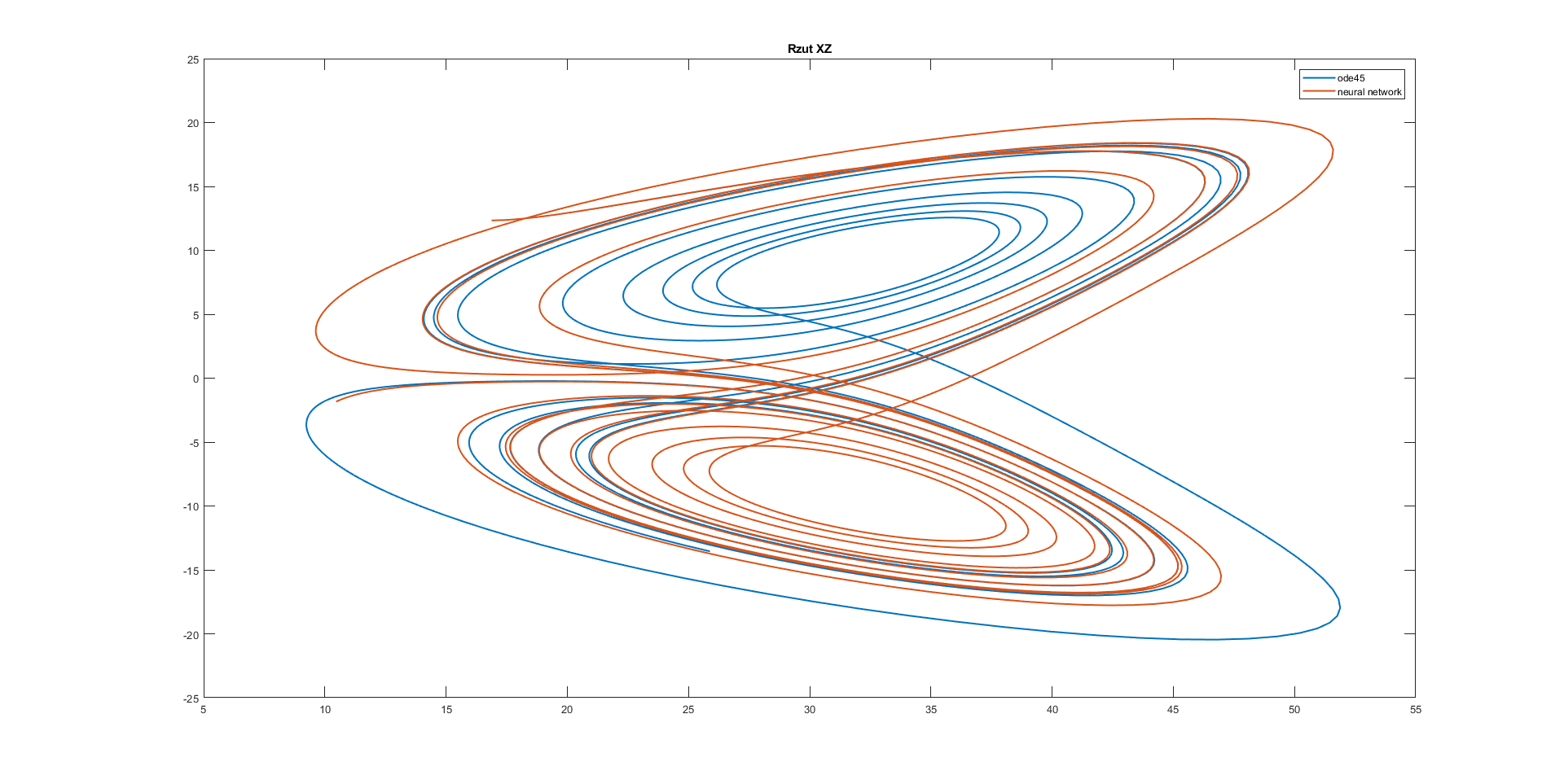
figure 
plot(y(:,3), y(:,1), ynn(:,3), ynn(:,1),'Linewidth',1.5)
legend('ode45','neural network');
title('Rzut XZ');

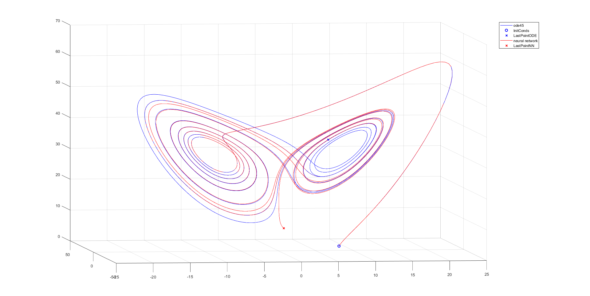
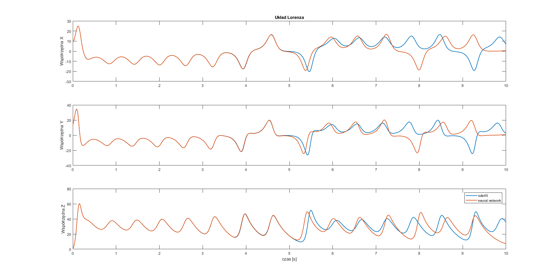
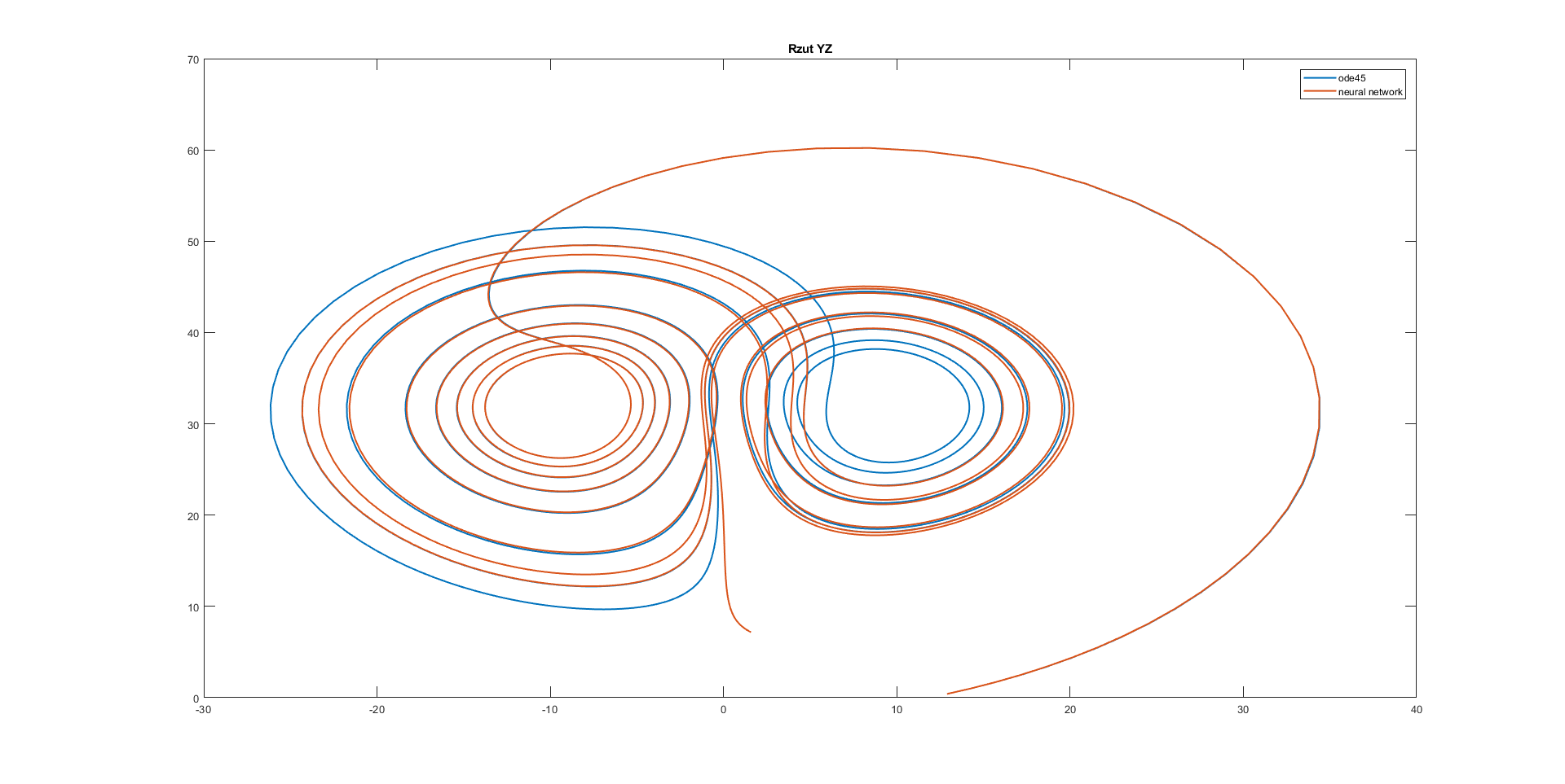
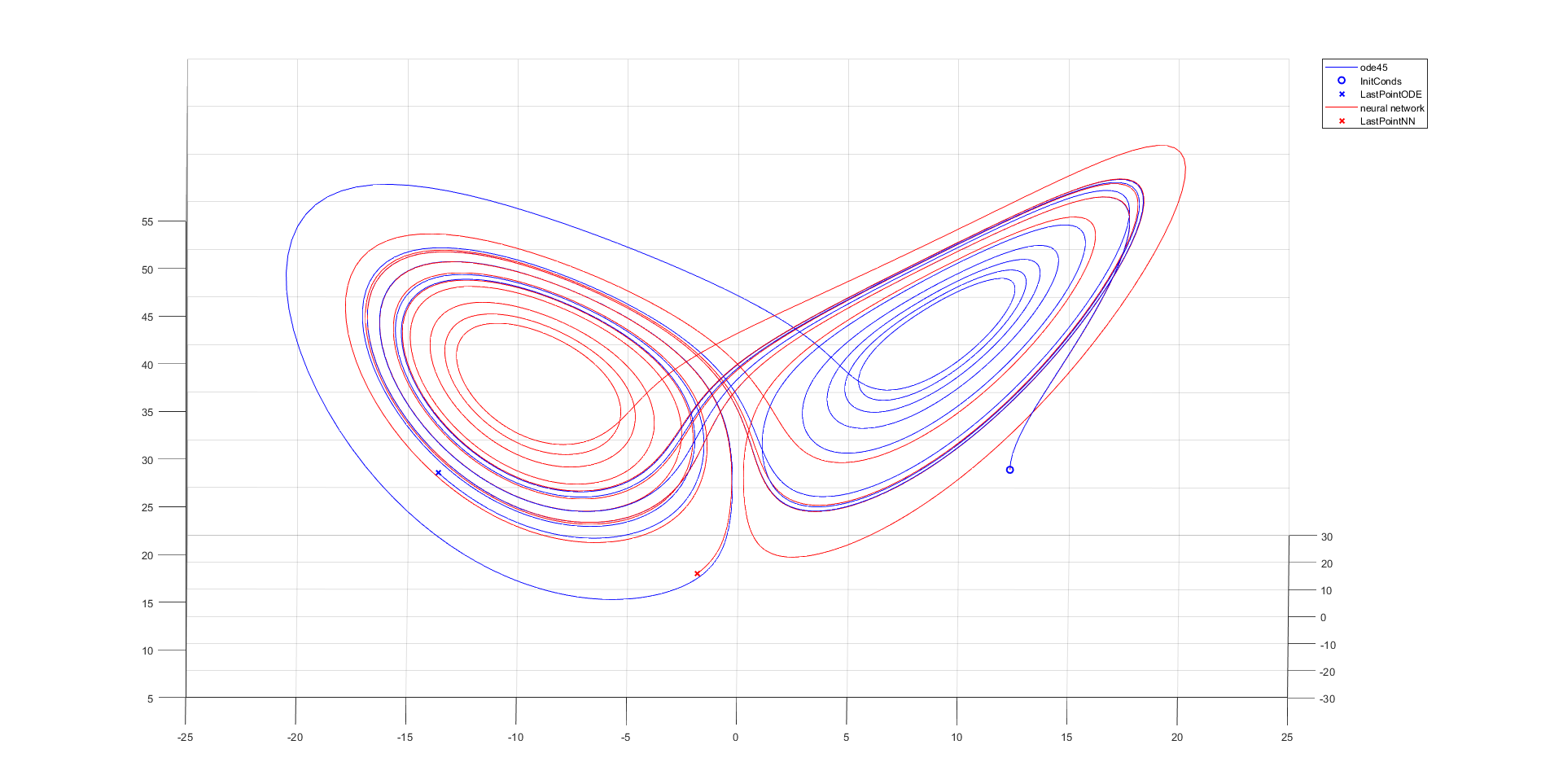
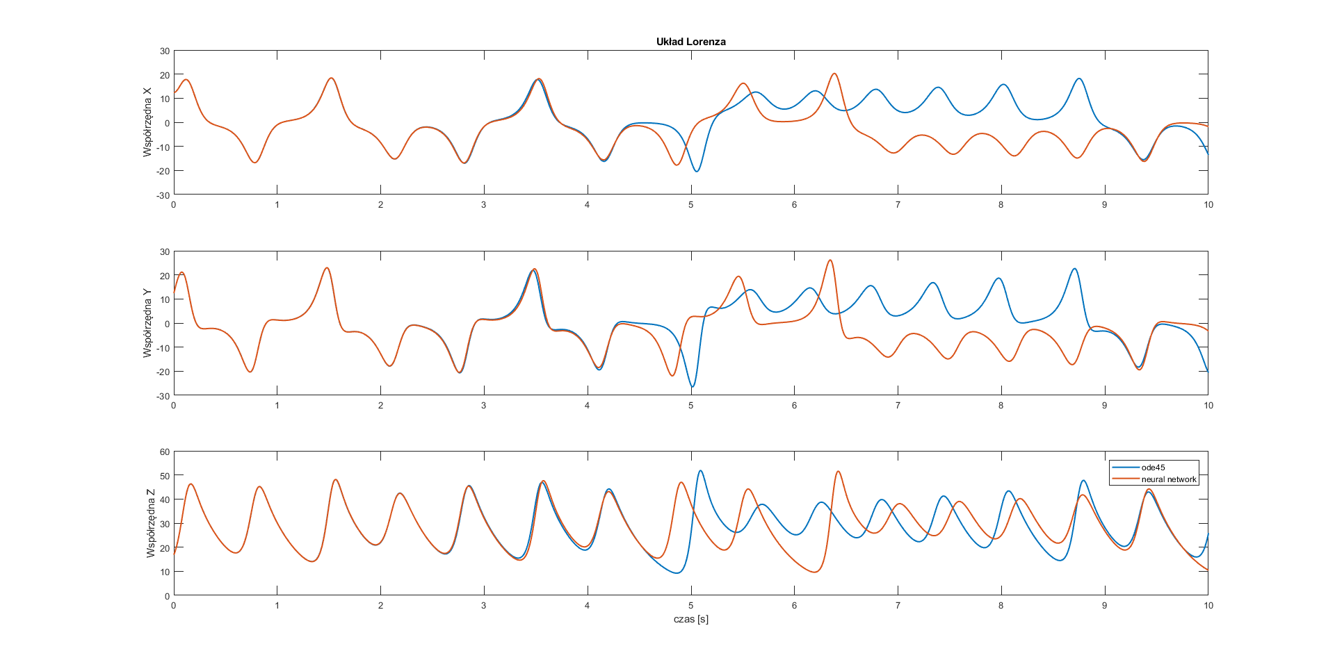
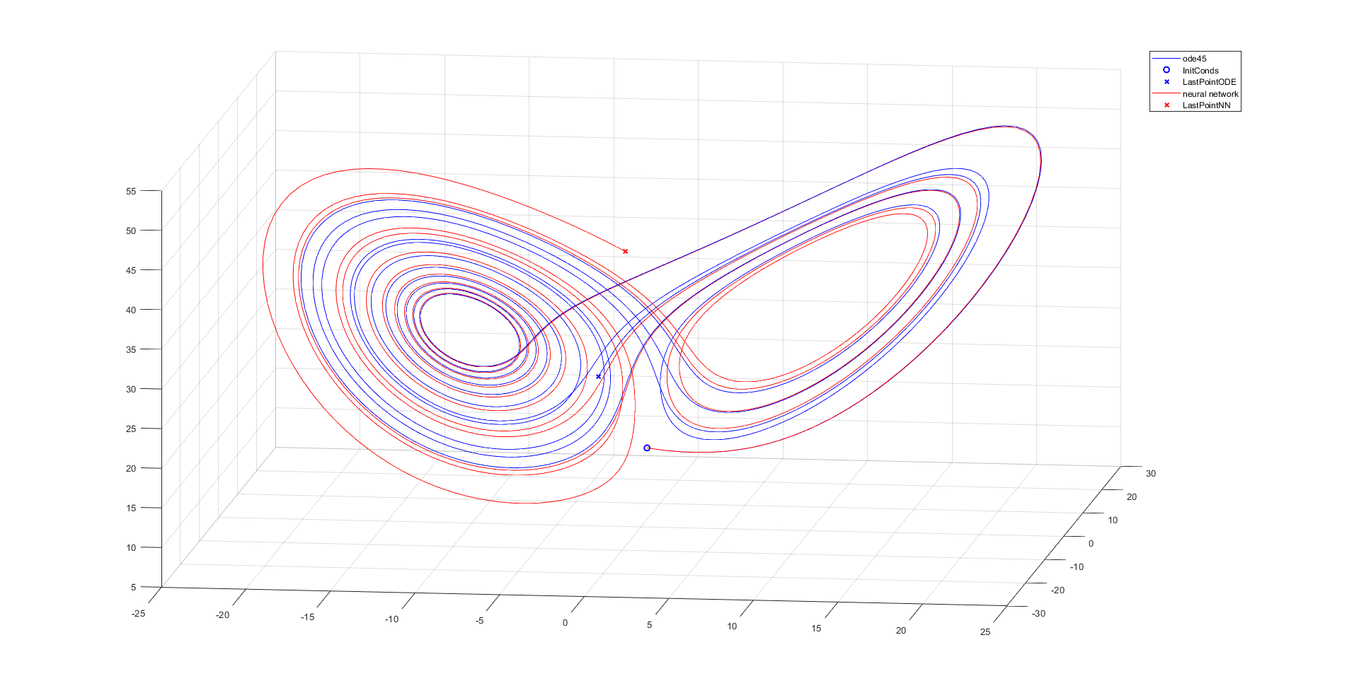
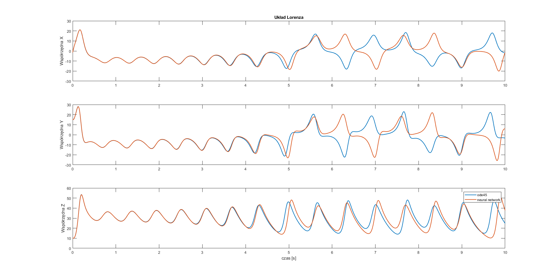
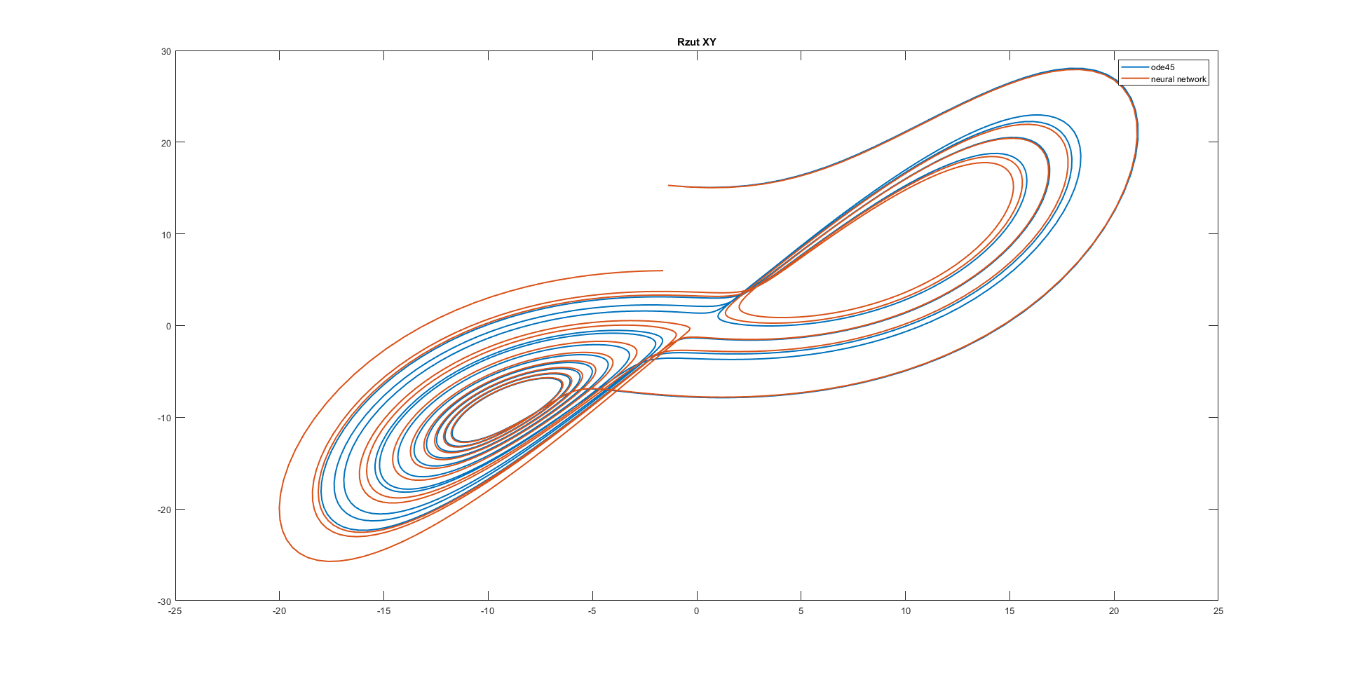
Conclusion: All of the used neural networks have good approximation for half of the considered time.
Next, the sequence of multilayer neural network layers is not insignificant. Intuition suggests using the sieve method — i.e. sieving the particles starting from the sieve with the largest mesh and ending with the smallest mesh. However, this is not a completely good approach when constructing a multilayer neural network. The 5-layer network has been arranged in this way — based on MSE. The question is whether the reverse arrangement should be considered optimal? In my opinion, in neural networks and general in artificial intelligence algorithms there are many randomities, many factors are chosen experimentally having no idea why the results are good at a given value of some coefficient, and bad at another its value. If the algorithm has such a large number of unknowns, it is impossible to give an unambiguous answer to the problem.

Moral: try to use mathematics instead.